McGinley Dynamic

Written by Miroslav Marinov

Miroslav Marinov

Miroslav Marinov, a financial news editor at TradingPedia, is engaged with observing and reporting on the tendencies in the Foreign Exchange Market, as currently his focus is set on the major currencies of eight developed nations worldwide.

, | Updated: September 15, 2025

Developed by John McGinley in 1990 and introduced in the Market Technicians Association’s Journal of Technical Analysis in 1997, the McGinley Dynamic indicator attempts to solve the lag problem that traditional simple and exponential moving averages encounter. It adjusts itself automatically to the speed of the market. The indicator is considered a price-smoothing mechanism that follows prices much more closely than any moving average. In this way, price separation and whipsaws are reduced to a minimum. The McGinley Dynamic (MD) indicator can be calculated as follows:

MD = MD1 + (Price – MD1) / (N * (Price / MD1) ^ 4), where

– MD1 refers to the previous value of the Dynamic indicator
– N is the Dynamic tracking factor

As a result of this calculation, the Dynamic line accelerates during bear trends as it follows prices, but moves more slowly during bull trends. In the formula above, the difference between the Dynamic and the price is divided by N times the ratio of the two, raised to the fourth power. This fourth power introduces an adjustment factor that increases more rapidly as the difference between the Dynamic and the current data becomes larger.

McGinley suggests that traditional moving averages and his Dynamic indicator should be used as smoothing mechanisms rather than as trading systems or signal providers. However, a trader can use the McGinley Dynamic in the same way that moving averages are generally used. On the chart below, the difference between the Dynamic and the 20-period Exponential Moving Average is visible.

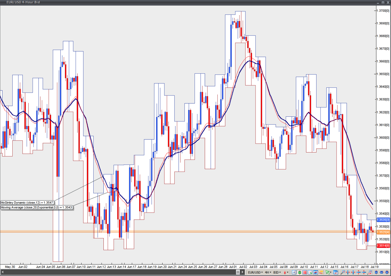
Chart source: VT Trader